Hello again! This is the follow-up blog post of the original Fantastic GANs and where to find them. If you haven’t checked that article or you are completely new to GANs, consider giving it a quick read - there’s a brief summary of the previous post ahead, though. It has been 8 months since the last post and GANs aren’t exactly known for being a field with few publications. In fact, I don’t think we are very far from having more types of GAN names than Pokémon. Even Andrej Karpathy himself finds it difficult to keep up to date:
GANs seem to improve on timescales of weeks; getting harder to keep track of. Another impressive paper and I just barely skimmed the other 3
— Andrej Karpathy (@karpathy) 4th of April 2017
So, having this in mind. Let’s see what relevant advances have happened in these last months.
What this post is not about
This is what you won’t find in this post:
- Complex technical explanations.
- Code (links to code for those interested, though).
- An exhaustive research list (you can already find one here).
What this post is about
- A summary of relevant topics about GANs, starting where I left it on the previous post.
- A lot of links to other sites, posts and articles so you can decide where to focus on.
Index
Refresher
Let’s get a brief refresher from the last post.
- What are GANs: two neural networks competing (and learning) against each other. Popular uses for GANs are generating realistic fake images, but they can also be used for unsupervised learning (e.g. learning features from data without labels).
 GANs in a nutshell.
- Relevant models from previous post:
- Generative Adversarial Networks: the original, vanilla, GANs.
- Deep Convolutional GANs (DCGANs): first major improvement on the GAN architecture in terms of training stability and quality of the samples.
- Improved DCGANs: another improvement over the previous DCGAN baseline. It allows generating higher-resolution images.
- Conditional GANs (cGANs): GANs that use label information to enhance the quality of the images and control how these images will look.
- InfoGANs: this type is able to encode meaningful image features in a completely unsupervised way. For example, on the digit dataset MNIST, they encode the rotation of the digit.
- Wasserstein GANs (WGANs): redesign of the original loss function, which correlates with image quality. This also improves training stability and makes WGANs less reliant on the network architecture.
GANs: the evolution (part II)
Here I’m going to describe in chronological order the most relevant GAN articles that have been published lately.
Improved WGANs (WGAN-GP)
TL;DR: take Wasserstein GANs and remove weight clipping - which is the cause of some undesirable behaviours - for gradient penalty. This results in faster convergence, higher quality samples and a more stable training.
The problem. WGANs sometimes generate poor quality samples or fail to converge in some settings. This is mainly caused by the weight clipping (clamping all weights into a range [min, max]) performed in WGANs as a measure to satisfy the Lipschitz constraint. If you don’t know about this constraint, just keep in mind that it’s a requirement for WGANs to work properly. Why is weight clipping a problem? Because it biases the WGAN to use much simpler functions. This means that the WGAN might not be able to model complex data with simple approximations (see image below). Additionally, weight clipping makes vanishing or exploding gradients prone to happen.
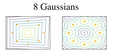 Here you can see how a WGAN fails to model 8 Gaussians (left) because it uses simple functions. On the other hand, a WGAN-GP correctly models them using more complex functions (right).
Gradient penalty. So how do we get rid of weight clipping? The authors of the WGAN-GP (where GP stands for gradient penalty) propose enforcing the Lipschitz constraint using another method called gradient penalty. Basically, GP consists of restricting some gradients to have a norm of 1. This is why it’s called gradient penalty, as it penalizes gradients which norms deviate from 1.
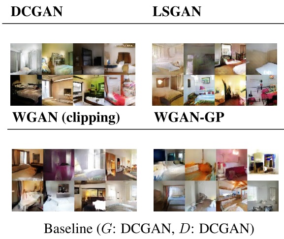
Advantages. As a result, WGANs trained using GP rather than weight clipping have faster convergence. Additionally, the training is much more stable to an extent where hyperparameter tuning is no longer required and the architecture used is not as critical. These WGAN-GP also generate high-quality samples, but it is difficult to tell by how much. On proven and tested architectures, the quality of these samples are very similar to the baseline WGAN:
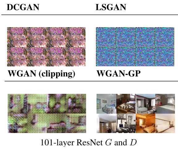
Where WGAN-GP is clearly superior is on generating high-quality samples on architectures where other GANs are prone to fail. For example, to the authors’ knowledge, it has been the first time where a GAN setting has worked on residual network architectures:
There are a lot of other interesting details that I had not mentioned, as it’d go far beyond the scope of this post. For those that want to know more (e.g. why the gradient penalty is applied just to “some” gradients or how to a apply this model to text), I recommend taking a look at the article.
You might want to use WGANs-GP if
you want an improved version of the WGAN which
- converges faster.
- works on a wide variety of architectures and datasets.
- doesn’t require as much hyperparameter tuning as other GANs.
Boundary Equilibrium GANs (BEGANs)
TL;DR: GANs using an auto-encoder as the discriminator. They can be successfully trained with simple architectures. They incorporate a dynamic term that balances both discriminator and generator during training.
Fun fact: BEGANs were published on the very same day as the WGAN-GP paper.
Idea. What sets BEGANs apart from other GANs is that they use an auto-encoder architecture for the discriminator (similarly to EBGANs) and a special loss adapted for this scenario. What is the reason behind this choice? Are auto-encoders not the devil as they force us to have a pixel reconstruction loss that makes blurry generated samples? To answer these questions we need to consider these two points:
-
Why reconstruction loss? The explanation from the authors is that we can rely on the assumption that, by matching the reconstruction loss distribution, we will also end up matching the real sample distributions.
-
Which leads us to: how? An important remark is that the reconstruction loss from the auto-encoder/discriminator (i.e. given this input image, give me the best reconstruction) is not the final loss that BEGANs are minimizing. This reconstruction loss is just a step to calculate the final loss. And the final loss is calculated using the Wasserstein distance (yes, it’s everywhere now) between the reconstruction loss on real and generated data.
This might be a lot of information at once but, once we see how this loss function is applied to the generator and discriminator, it’ll be much clearer:
- The generator focuses on generating images that the discriminator will be able to reconstruct well.
- The discriminator tries to reconstruct real images as good as possible while reconstructing generated images with the maximum error.
Diversity factor. Another interesting contribution is what they call the diversity factor. This factor controls how much you want the discriminator to focus on getting a perfect reconstruction on real images (quality) vs distinguish real images from generated (diversity). Then, they go one step further and use this diversity factor to maintain a balance between the generator and discriminator during training. Similarly to WGANs, they use this equilibrium between both networks as a measure of convergence that correlates with image quality. However, unlike WGANs (and WGANs-GP), they use Wasserstein distance in such a way that the Lipschitz constrain is not required.
Results. BEGANs do not need any fancy architecture to train properly; as mentioned in the paper: “no batch normalization, no dropout, no transpose convolutions and no exponential growth for convolution filters”. The quality of the generated samples (128x128) is quite impressive*:
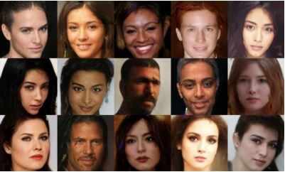
*However, there’s an important detail to be considered in this paper. They are using an unpublished dataset which is almost twice the size of the widely used CelebA dataset. Then, for a more realistic qualitative comparison, I invite you to check any public implementation using CelebA and see the generated samples.
As a final note, if you want to know more about BEGANs, I recommend reading this blog post, which goes much more into detail.
You might want to use BEGANs…
… for the same reasons you would use WGANs-GP. They both offer very similar results (stable training, simple architecture, loss function correlated to image quality), they mainly differ in their approach. Due to the hard nature of evaluating generative models, it’s difficult to say which is better. As Theis et al. says in their paper, you should choose a evaluation method or another depending on the application. In this case, WGAN-GP has a better Inception score and yet BEGANs generate very high-quality samples. Both are innovative and promising.
Progressive growing of GANs (ProGANs)
TL;DR: Progressively add new high-resolution layers during training that generate incredibly realistic images. Other improvements and a new evaluation method are also proposed. The quality of the generated images is astonishing.
Generating high-resolution images is a big challenge. The larger the image, the easier is for the network to fail because it needs to learn to generate more subtle and complex details. To give a little bit of context, before this article, realistic generated images were around 256x256. Progressive GANs (ProGANs) take this to a whole new level by successfully generating completely realistic 1024x1024 images. Let’s see how.
Idea. ProGANs, which are built upon WGANs-GP, introduce a smart way to progressively add new layers on training time. Each one of these layers upsamples the images to a higher resolution for both the discriminator and generator. Let’s go step by step:
- Start with the generator and discriminator training with low-resolution images.
- At some point (e.g. when they start to converge) increase the resolution. This is done very elegantly with a “transition period” / smoothing:
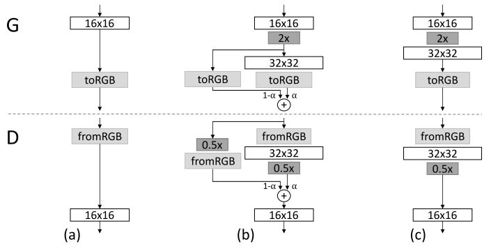
Instead of just adding a new layer directly, it's added on small linear steps controlled by α.
Let's see what happens in the generator. At the beginning, when α = 0, nothing changes. All the contribution of the output is from the previous low-resolution layer (16x16). Then, as α is increased, the new layer (32x32) will start getting its weights adjusted through backpropagation. By the end, α will be equal to 1, meaning that we can totally drop the "shortcut" used to skip the 32x32 layer. The same happens to the discriminator, but the other way around: instead of making the image larger, we make it smaller.
- Once the transition is done, keep training the generator and discriminator. Go to step 2 if the resolution of currently generated images is not the target resolution.
But, wait a moment… isn’t this upsampling and concatenation of new high-resolution images something already done in StackGANs (and the new StackGANs++)? Well, yes and no. First of all, StackGANs are text-to-image conditional GANs that use text descriptions as an additional input while ProGANs don’t use any kind of conditional information. But, more interestingly, despite both StackGANs and ProGANs using concatenation of higher resolution images, StackGANs require as many independent pairs of GANs — which need to be trained separately — per upsampling. Do you want to upsample 3 times? Train 3 GANs. On the other hand, in ProGANs only a single GAN is trained. During this training, more upsampling layers are progressively added to upsample the images. So, the cost of upsampling 3 times is just adding more layers on training time, as opposed to training from scratch 3 new GANs. In summary, ProGANs use a similar idea from StackGANs and they manage to pull it off more elegantly, with better results and without extra conditional information.
Results. As a result of this progressive training, generated images in ProGANs are of higher quality and training time is reduced by 5.4x on 1024x1024 images. The reasoning behind this is that a ProGAN doesn’t need to learn all large-scale and small-scale representations at once. In a ProGAN, first the small-scale are learnt (i.e. low-resolution layers converge) and then the model is free to focus on refining purely the large-scale structures (i.e. new high-resolution layers converge).
Other improvements. Additionally, the paper proposes new design decisions to further improve the performance of the model. I’ll briefly describe them:
-
Minibatch standard deviation: encourages each minibatch to have similar statistics using the standard deviation over all features of the minibatch. This is then summarized as a single value in a new layer that is inserted towards the end of the network.
-
Equalized learning rate: makes sure that the learning speed is the same for all weights by dividing each weight by a constant continuously during training.
-
Pixelwise normalization: on the generator, each feature vector is normalized after each convolutional layer (exact formula in the paper). This is done to prevent the magnitudes of the gradients of the generator and discriminator from escalating.
CelebA-HQ. As a side note, it is worth mentioning that the authors enhanced and prepared the original CelebA for high-resolution training. In a nutshell, they remove artifacts, apply a Gaussian filtering to produce a depth-of-field effect, and detect landmarks on the face to finally get a 1024x1024 crop. After this process, they only keep the best 30k images out of 202k.
Evaluation. Last but not least, they introduce a new evaluation method:
- The idea behind it is that the local image structure of generated images should match the structure of the training images.
- How do we measure local structure? With a Laplacian pyramid, where you get different levels of spatial frequency bands that can be used as descriptors.
- Then, we extract descriptors from the generated and real images, normalize them, and check how close they are using the famous Wasserstein distance. The lower the distance, the better.
You might want to use ProGANs…
- If you want state-of-the-art results. But consider that…
- … you will need a lot of time to train the model: “We trained the network on a single NVIDIA Tesla P100 GPU for 20 days”.
- If you want to start questioning your own reality. Next GAN iterations might create more realistic samples than real life.
Honorable mention: Cycle GANs
Cycle GANs are, at the moment of writing these words, the most advanced image-to-image translation using GANs. Tired that your horse is not a zebra? Or maybe that Instagram photo needs more winter? Say no more.

These GANs don’t require paired datasets to learn to translate between domains, which is good because this kind of data is very difficult to obtain. However, Cycle GANs still need to be trained with data from two different domains X and Y (e.g. X: horses, Y: zebras). In order to constrain the translation from one domain to another, they use what they call a “cycle consistent loss”. This basically means that if you translate a horse A into a zebra A, transforming the zebra A back to a horse should give you the original horse A as a result.
This mapping from one domain to another is different from the also popular neural style transfer. The latter combines the content of one image with the style of another, whilst Cycle GANs learn a high level feature mapping from one domain to another. As a consequence, Cycle GANs are more general and can also be used for all sorts of mappings such as converting a sketch of an object into a real object.

Let’s recap. We have had two major improvements, WGANs-GP and BEGANs. Despite following different research directions, they both offer similar advantages. Then, we have ProGANs (based on WGANs-GP), which unlock a clear path to generate realistic high-resolution images. Meanwhile, CycleGANs reminds us about the power of GANs to extract meaningful information from a dataset and how this information can be transferred to another unrelated data distribution.
Other useful resources
Here are a bunch of links to other interesting posts:
- GAN playground: this is the most straightforward way to play around GANs. Simply click the link, set up some hyperparameters and train a GAN in your browser.
- Every paper and code: here’s a link to all GAN related papers sorted by the number of citations. It also includes courses and Github repos. Very recommended, but the last update was on July 2017.
- GANs timeline: similar to the previous link, but this time every paper is ordered according to publishing date.
- GANs comparison: in this link, different versions of GANs are tested without cherry picking. This is a important remark, as generated images shown in publications might not be really representative of the overall performance of the model.
- Some theory behind GANs: in a similar way to this post, this link contains some nice explanations of the theory (especially the loss function) of the main GAN models.
- High-resolution generated images: this is more of a curiosity, but here you can actually see how 4k x 4k generated images actually look like.
- Waifus generator: you’ll never feel alone ever again ( ͡° ͜ʖ ͡°)

Hope this post has been useful and thanks for reading! I want to also say thanks to Blair Young for his feedback on this post. If you think there’s something wrong, inaccurate or want to make any suggestion, please let me know in the comment section below or in this reddit thread.
Oh, and I have just created my new twitter account. I’ll be sharing my new blog posts there.